set.seed(1234)

library(tidyverse)Introduction to Exponential Random Graph Models
Understanding Network Structure with the Enemy’s Enemy Principle
ERGM
Network analysis
What is an ERGM?
Imagine you observe some network — for example, countries at war with each other. You want to learn why this network looks the way it does. An ERGM provides the following answer: “Some network patterns are more likely than others, and I can explain why by looking at their specific features”.
Why Networks and ERGMs Matter for Political Science
One core problem with using standard statistical methods, like regression, to study connections between countries, organizations, or people is that these methods assume each relationship is independent of every other. For instance, they treat the relationship between the US and France as if it exists in isolation, completely unaffected by the US’s relationship with Germany. This assumption is fundamentally inaccurate in real-world political and social systems, where ties influence each other.
Exponential Random Graph Models (ERGMs) are a specialized set of statistical techniques designed to analyze networks by recognizing and modeling these complex interdependencies. They look for and quantify common patterns that emerge when relationships influence one another, such as reciprocity (if A links to B, B is likely to link back to A) or transitivity (if A links to B, and B links to C, then A is likely to link to C). This allows researchers to study how the overall structure of the network, not just individual factors, drives the formation of new connections. By doing this, ERGMs offer a more accurate and realistic framework than methods that treat all connections as standalone events.
The Basic Logic
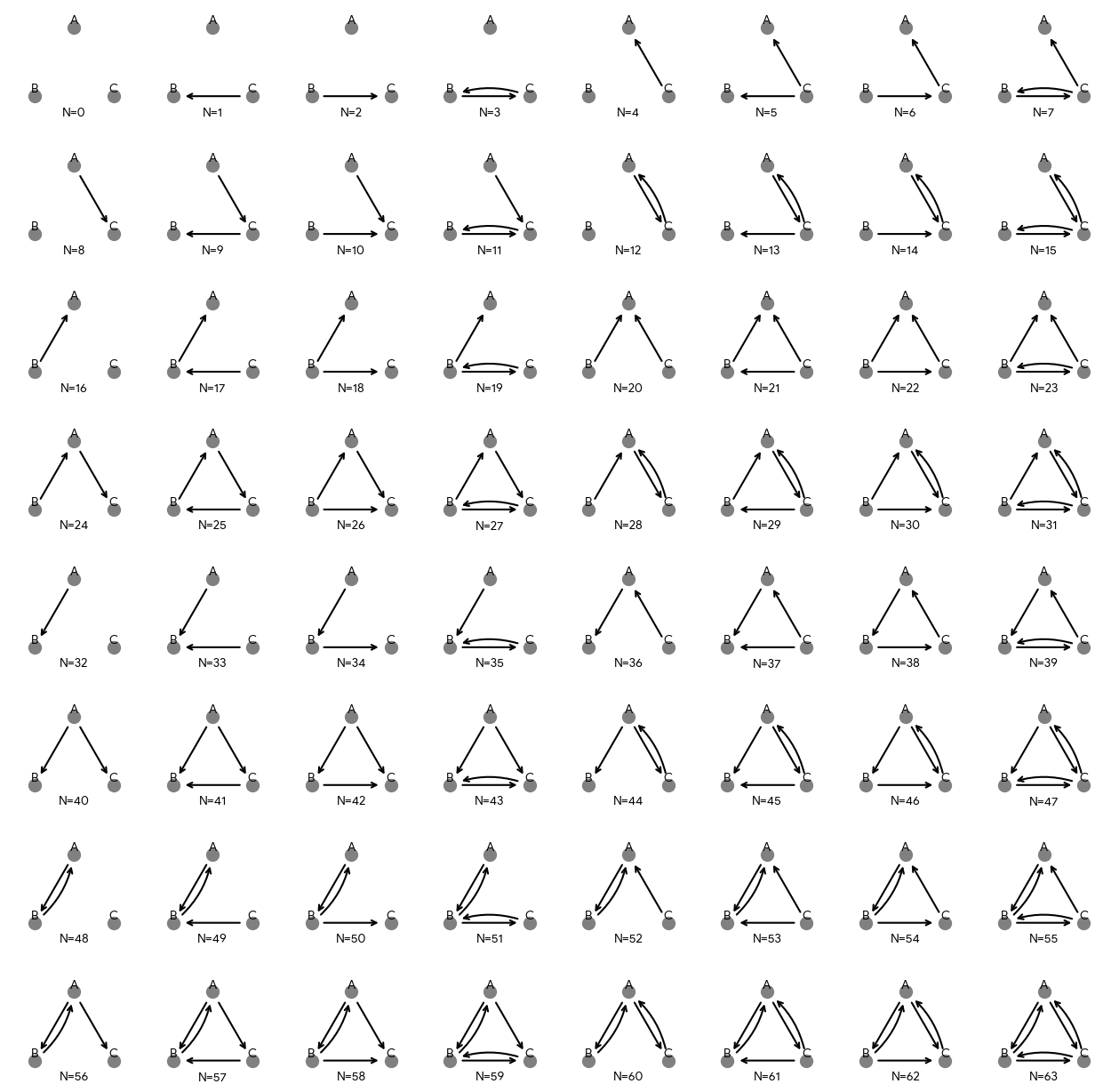
Start with all possible networks that could form between your actors. For example, if you have three actors (all of which can both send and receive ties), 64 directed networks could form between them.
Next, assign each of these possible networks some probability based on its features. For example, imagine that each of the above networks represents a different configuration of who is at war with whom. We might find that:
- Networks where democracies fight other democracies might be LESS likely (democratic peace theory)
- Networks where geographically distant countries fight might be LESS likely
- Networks where strong countries attack weak ones might be MORE likely
Networks with more “desirable” features receive a higher probability. Those with less “desirable” features receive a lower probability. The parameters (β values) tell you how much each feature matters.
Predicting International Conflict
Let’s work through a concrete example. Imagine you would like to work out what features shape the likelihood of war breaking out. You know the following features matter:
Democracy: Whether two countries are both democracies (if yes, they are less likely to go to war with each other)
Distance: The distance between their capital cities (war becomes less likely with distance)
Military strength: Their relative strength (stronger countries are more likely to attack weaker ones)
Avoiding multi-front wars: If A fights B, and B fights C, then A is less likely to also fight C (countries avoid complex triangular conflicts and instead form coalitions)
We will examine a hypothetical world of three countries in which these four feature are the only significant determinants of one country starting a war with another. Further, we will know just how much each feature matters to this decision. Knowing this allows us to see how ERGMs work. We can then move on to the more useful research project of discovering these parameters.
Why Three Nodes?
The number of possible networks grows exponentially with the number of nodes. With three nodes, we have a manageable 64 possible networks that we can enumerate completely. This lets us understand the mechanics of ERGMs before tackling larger networks that require simulation methods.
Step 1: Define Node Attributes
Let’s set up our known world of three countries:
nodes <- tibble(
  node = c("A", "B", "C"),
  democracy = c(1, 1, 0),     # A and B are democracies, C is not
  cinc = c(.142, .07, .04)    # Composite Index of National Capability
)

knitr::kable(nodes)| node | democracy | cinc |
|---|---|---|
| A | 1 | 0.142 |
| B | 1 | 0.070 |
| C | 0 | 0.040 |
What do these variables mean?
democracy: A value of 1 means the country is a democracy, 0 means it is not. In our world, countries A and B are democracies, while C is not.cinc: This is the Composite Index of National Capability, which measures a country’s military power. It ranges from 0 to 1, with higher values indicating greater military capability. In our example, A is the strongest (0.142), followed by B (0.07), then C (0.04).
Step 2: Create All Possible Directed Ties (Dyads)
For a three-node directed network, we have 3 × 2 = 6 possible ties. Each of our three nodes can send a tie (initiate war) to two other nodes.
dyads <- expand_grid(
  node_1 = nodes$node,
  node_2 = nodes$node
) %>%
  filter(node_1 != node_2) %>%  # Remove self-loops
  left_join(rename_with(nodes, ~ paste0(.x, "_1")),
            by = "node_1") %>%
  left_join(rename_with(nodes, ~ paste0(.x, "_2")),
            by = "node_2") %>%
  transmute(
    node_1, node_2,

    # Covariate 1: Both nodes are democracies
    both_democracy = as.numeric(democracy_1 == 1 & democracy_2 == 1),

    # Covariate 2: CINC ratio (sender/receiver)
    cinc_ratio = cinc_1 / cinc_2,

    # Covariate 3: Distance between capitals in thousands of kms
    dist = c(12, 40, 12, 35, 40, 35)
  )

knitr::kable(dyads)| node_1 | node_2 | both_democracy | cinc_ratio | dist |
|---|---|---|---|---|
| A | B | 1 | 2.0285714 | 12 |
| A | C | 0 | 3.5500000 | 40 |
| B | A | 1 | 0.4929577 | 12 |
| B | C | 0 | 1.7500000 | 35 |
| C | A | 0 | 0.2816901 | 40 |
| C | B | 0 | 0.5714286 | 35 |
Understanding the covariates:
both_democracy: This equals 1 if bothnode_1andnode_2are democracies. In our example, this is true for A→B and B→A. We expect these dyads to be less likely to go to war.cinc_ratio: This is the military capability ofnode_1divided bynode_2. Values greater than 1 mean the potential attacker is stronger. For example, A→C has a ratio of 3.55, meaning A is much stronger than C.dist: Distance between capitals in thousands of kilometers. Greater distances should make war less likely.
Step 3: Define the “True” ERGM Parameters
We’re going to set up a known world where we specify exactly how each feature affects the probability of war. In real research, we would estimate these parameters from data, but here we’ll define them to understand how ERGMs work.
true_beta_0 <- -2.0   # Baseline
true_beta_1 <- -3.5   # Both democracy effect
true_beta_2 <- 1.5    # CINC ratio effect
true_beta_3 <- -0.05  # Distance effect
true_beta_4 <- -2.0   # Transitive triads effect
Interpreting each parameter:
β₀ = -2.0 (Baseline): This negative number means wars are generally rare. If we ignore all other features, countries don’t randomly fight — there needs to be a reason.
β₁ = -3.5 (Both Democracy): This large negative number means when both countries are democracies, war becomes much less likely. This captures the democratic peace theory.
β₂ = 1.5 (CINC Ratio): This positive number means stronger countries are more likely to attack weaker ones. Higher military advantage increases the probability of war.
β₃ = -0.05 (Distance): This negative number means farther countries are less likely to fight. Geography creates a barrier to conflict.
β₄ = -2.0 (Transitive Triads): This is our structural parameter. It captures patterns of conflict clustering, which we’ll explain next.
Understanding the Structural Feature: Transitive Triads
ERGMs allow us to capture features that shape the likelihood of some outcome other than those that depend only on the two countries involved in a potential war (A and B’s attributes, their distance, etc.). For example, the transitive triads parameter is different — it depends on the entire network structure. We cannot use traditional dyadic data structures to estimate its influence on conflict.
What is a transitive triad?
A transitive triad exists when three countries form a directed triangle of conflict:
A is at war with B (A→B exists)
B is at war with C (B→C exists)
A is at war with C (A→C exists)
This forms a complete cycle where each country that fights another country also fights that country’s enemy.
Why does this matter?
In reality, transitive triads are rare in international conflict. Here’s why:
If the United States fights Russia, and Russia fights Ukraine, the United States typically does not fight Ukraine. Instead, the U.S. often supports Ukraine (the principle: “the enemy of my enemy is my friend”).
Countries tend to form coalitions against common enemies rather than creating triangular wars. When A fights B, and B fights C, A and C more often become allies than enemies.
The key insight: With β₄ = -2.0 (negative), networks that contain transitive triads are less probable. Countries avoid getting into complex multi-front wars. This one parameter changes the entire distribution of likely networks by discouraging clustered conflict patterns.
Step 4: Calculate Network Probabilities
Here’s where ERGMs with structural features become different. We cannot simply calculate the probability of each tie independently. Why? Because whether A→C exists depends on whether A→B and B→C exist!
The solution: We must look at all 64 possible complete networks and calculate the probability of each entire network configuration.
Generate All Possible Networks
all_networks <- expand_grid(
  tie_AB = 0:1, tie_AC = 0:1, tie_BA = 0:1,
  tie_BC = 0:1, tie_CA = 0:1, tie_CB = 0:1
) %>%
  mutate(network_id = row_number())

all_networks
# A tibble: 64 × 7
tie_AB tie_AC tie_BA tie_BC tie_CA tie_CB network_id
<int> <int> <int> <int> <int> <int> <int>
1 0 0 0 0 0 0 1
2 0 0 0 0 0 1 2
3 0 0 0 0 1 0 3
4 0 0 0 0 1 1 4
5 0 0 0 1 0 0 5
6 0 0 0 1 0 1 6
7 0 0 0 1 1 0 7
8 0 0 0 1 1 1 8
9 0 0 1 0 0 0 9
10 0 0 1 0 0 1 10
# ℹ 54 more rowsEach row represents one possible network. For example:
Row 1:
tie_AB = 0, tie_AC = 0, ..., tie_CB = 0(empty network, no wars)Row 64:
tie_AB = 1, tie_AC = 1, ..., tie_CB = 1(complete network, all at war)
Calculate Sufficient Statistics for Each Network
For each possible network, we need to count:
- How many wars exist (edges)
- How many wars involve two democracies
- Sum of CINC ratios across all wars
- Sum of distances across all wars
- How many transitive triads exist (the structural feature)
What are sufficient statistics?
Sufficient statistics are summary measures of a network that contain all the information needed to calculate the network’s probability under an ERGM.
Rather than tracking every individual tie separately, sufficient statistics reduce the network to a few key counts that capture what the model cares about. These five statistics are “sufficient” because two networks with identical sufficient statistics have identical probabilities under the model, even if the specific ties differ.
Why “sufficient”?
For example, suppose:
- Network A has wars A→B and C→D (two wars between non-democracies)
- Network B has wars A→C and B→D (two different wars between non-democracies)
If both networks have the same sufficient statistics (same number of edges, same democracy pairs, same total CINC ratios, same total distances, same transitive triads), they receive the same probability—the model only cares about the aggregate counts, not which specific countries fight which others.
Now let’s calculate these statistics:
network_stats <- all_networks %>%
  rowwise() %>%
  mutate(
    # Sufficient statistic 1: Number of edges (wars)
    n_edges = sum(c(tie_AB, tie_AC, tie_BA, tie_BC, tie_CA, tie_CB)),

    # Sufficient statistic 2: Wars where both are democracies
    n_both_dem = tie_AB * dyads$both_democracy[1] +  # A→B
                 tie_BA * dyads$both_democracy[3],   # B→A

    # Sufficient statistic 3: Sum of CINC ratios
    sum_cinc = tie_AB * dyads$cinc_ratio[1] +  # A→B
               tie_AC * dyads$cinc_ratio[2] +  # A→C
               tie_BA * dyads$cinc_ratio[3] +  # B→A
               tie_BC * dyads$cinc_ratio[4] +  # B→C
               tie_CA * dyads$cinc_ratio[5] +  # C→A
               tie_CB * dyads$cinc_ratio[6],   # C→B

    # Sufficient statistic 4: Sum of distances
    sum_dist = tie_AB * dyads$dist[1] +
               tie_AC * dyads$dist[2] +
               tie_BA * dyads$dist[3] +
               tie_BC * dyads$dist[4] +
               tie_CA * dyads$dist[5] +
               tie_CB * dyads$dist[6],

    # Sufficient statistic 5: Number of transitive triads
    # Count patterns where i→j AND j→k AND i→k all exist
    n_transitive = (tie_AB * tie_BC * tie_AC) +  # A→B→C (and A→C)
                   (tie_AC * tie_CB * tie_AB) +  # A→C→B (and A→B)
                   (tie_BA * tie_AC * tie_BC) +  # B→A→C (and B→C)
                   (tie_BC * tie_CA * tie_BA) +  # B→C→A (and B→A)
                   (tie_CA * tie_AB * tie_CB) +  # C→A→B (and C→B)
                   (tie_CB * tie_BA * tie_CA)    # C→B→A (and C→A)
  ) %>%
  ungroup()

select(network_stats, network_id:n_transitive)
# A tibble: 64 × 6
network_id n_edges n_both_dem sum_cinc sum_dist n_transitive
<int> <int> <dbl> <dbl> <dbl> <int>
1 1 0 0 0 0 0
2 2 1 0 0.571 35 0
3 3 1 0 0.282 40 0
4 4 2 0 0.853 75 0
5 5 1 0 1.75 35 0
6 6 2 0 2.32 70 0
7 7 2 0 2.03 75 0
8 8 3 0 2.60 110 0
9 9 1 1 0.493 12 0
10 10 2 1 1.06 47 0
# ℹ 54 more rowsCalculate Network Probabilities Using the ERGM Formula
The probability of each network is given by:
\[P(\text{Network} \mid \theta) = \frac{\exp(\theta' \cdot s(\text{Network}))}{\kappa(\theta)}\]
Where:
\(\theta\) = our parameters (β₀, β₁, β₂, β₃, β₄)
\(s(\text{Network})\) = sufficient statistics for that network
\(\kappa(\theta)\) = normalizing constant (ensures probabilities sum to 1 by being the sum of all network scores)
In plain language: “The probability of a network equals its score divided by the sum of all possible networks’ scores.”
# Calculate the unnormalized log-probability for each network
network_stats <- network_stats %>%
  mutate(
    log_prob_unnorm = true_beta_0 * n_edges +
                      true_beta_1 * n_both_dem +
                      true_beta_2 * sum_cinc +
                      true_beta_3 * sum_dist +
                      true_beta_4 * n_transitive
  )

# Calculate the normalizing constant
log_kappa <- log(sum(exp(network_stats$log_prob_unnorm)))

# Calculate final probabilities
network_stats <- network_stats %>%
  mutate(
    log_prob = log_prob_unnorm - log_kappa,
    prob = exp(log_prob)
  ) %>%
  arrange(desc(prob))

select(network_stats, network_id, log_prob_unnorm, log_prob, prob)
# A tibble: 64 × 4
network_id log_prob_unnorm log_prob prob
<int> <dbl> <dbl> <dbl>
1 17 1.32 -0.639 0.528
2 21 0.200 -1.76 0.171
3 1 0 -1.96 0.140
4 5 -1.12 -3.09 0.0455
5 18 -1.57 -3.53 0.0292
6 49 -1.73 -3.70 0.0248
7 19 -2.25 -4.22 0.0147
8 22 -2.69 -4.66 0.00949
9 2 -2.89 -4.86 0.00777
10 33 -3.06 -5.02 0.00659
# ℹ 54 more rows
Understanding the log space calculations
You might wonder why we use log_prob = log_prob_unnorm - log_kappa instead of directly calculating probabilities. Here’s why:
The mathematical identity:
- We want: P = exp(score) / κ(θ)
- Taking logs: log(P) = log(exp(score)) - log(κ(θ)) = score - log(κ(θ))
Why work in log space?
- Network probabilities can be extremely small (like 0.0000001)
- Computers can’t reliably store very small numbers (they “underflow” to exactly 0)
- But computers can store log(0.0000001) = -16.1 reliably
- We only convert back to regular probabilities at the end:
prob = exp(log_prob)
The calculation steps:
log_prob_unnorm= the score for each network (sum of β × statistics)log_kappa= log of the sum of all exponential scoreslog_prob= normalized log-probability = score - log(normalizing constant)prob= convert back to regular probability scale
Verify probabilities sum to 1:
sum(network_stats$prob)[1] 1Perfect! This confirms our probability distribution is valid.
Step 5: Examine the Most Likely Networks
network_stats %>%
  select(network_id, n_edges, n_both_dem, n_transitive, sum_cinc, sum_dist,
         prob) %>%
  slice(1:10) %>%
  mutate(prob_pct = scales::percent(prob, accuracy = 0.01)) %>%
  select(-prob) %>%
knitr::kable()| network_id | n_edges | n_both_dem | n_transitive | sum_cinc | sum_dist | prob_pct |
|---|---|---|---|---|---|---|
| 17 | 1 | 0 | 0 | 3.5500000 | 40 | 52.76% |
| 21 | 2 | 0 | 0 | 5.3000000 | 75 | 17.13% |
| 1 | 0 | 0 | 0 | 0.0000000 | 0 | 14.02% |
| 5 | 1 | 0 | 0 | 1.7500000 | 35 | 4.55% |
| 18 | 2 | 0 | 0 | 4.1214286 | 75 | 2.92% |
| 49 | 2 | 1 | 0 | 5.5785714 | 52 | 2.48% |
| 19 | 2 | 0 | 0 | 3.8316901 | 80 | 1.47% |
| 22 | 3 | 0 | 0 | 5.8714286 | 110 | 0.95% |
| 2 | 1 | 0 | 0 | 0.5714286 | 35 | 0.78% |
| 33 | 1 | 1 | 0 | 2.0285714 | 12 | 0.66% |
What do we notice?
The most probable networks tend to have:
Few edges (wars are rare, β₀ is negative)
Low or zero democracy pairs fighting (β₁ is very negative)
Few or no transitive triads (countries avoid multi-front wars, β₄ is negative)
When wars occur, they tend to be between strong and weak countries at close distances
Step 6: Simulate a Network from This Distribution
Now that we have probabilities for all 64 networks, we can randomly sample one network according to these probabilities. This is like the “data generating process” — it shows us what networks we’d expect to observe given our parameters.
# Sample one network according to probabilities
sampled_network_id <- sample(network_stats$network_id,
                              size = 1,
                              prob = network_stats$prob)

sampled_network <- network_stats %>%
  filter(network_id == sampled_network_id)
Our sampled network:
sampled_network %>%
  select(network_id:n_transitive, prob) %>%
knitr::kable()| network_id | n_edges | n_both_dem | sum_cinc | sum_dist | n_transitive | prob |
|---|---|---|---|---|---|---|
| 17 | 1 | 0 | 3.55 | 40 | 0 | 0.5276205 |
Which specific wars exist?
ties_list <- sampled_network %>%
  select(tie_AB, tie_AC, tie_BA, tie_BC, tie_CA, tie_CB) %>%
  pivot_longer(everything(), names_to = "tie", values_to = "exists") %>%
  filter(exists == 1) %>%
  mutate(tie = str_replace(tie, "tie_", ""),
         tie = paste0(str_sub(tie, 1, 1), "→", str_sub(tie, 2, 2)))

if (nrow(ties_list) > 0) {
  cat("Wars in this network:\n")
  print(ties_list$tie)
} else {
  cat("Empty network - no wars\n")
}
Wars in this network:
[1] "A→C"Understanding the Impact of Network Structure
What Does the Transitivity Parameter Mean?
Our parameter β₄ = -2.0 means that each additional transitive triad multiplies the probability of a network by \(\exp(-2.0) \approx 0.14\) (or divides it by about 7.4).
Concrete example:
Imagine two networks that are identical in every way except:
Network 1 has 0 transitive triads
Network 2 has 1 transitive triad
Network 2 is only 14% as probable as Network 1! Or equivalently, Network 1 is 7.4 (1 / 0.14) times more probable than Network 2.
Comparing With and Without Structure
Let’s see how the structural parameter changes things. We’ll calculate probabilities of each network with and without the transitivity term.
# Calculate probabilities WITHOUT transitivity
network_stats_no_struct <- network_stats %>%
  mutate(
    log_prob_unnorm_no_struct = true_beta_0 * n_edges +
                                true_beta_1 * n_both_dem +
                                true_beta_2 * sum_cinc +
                                true_beta_3 * sum_dist
                                # Note: NO β₄ term!
  )

log_kappa_no_struct <- log(sum(exp(network_stats_no_struct$log_prob_unnorm_no_struct)))

network_stats_no_struct <- network_stats_no_struct %>%
  mutate(
    log_prob_no_struct = log_prob_unnorm_no_struct - log_kappa_no_struct,
    prob_no_struct = exp(log_prob_no_struct)
  )
Top 10 networks WITH transitivity:
network_stats %>%
  select(network_id, n_edges, n_transitive, prob) %>%
  slice(1:10) %>%
  mutate(prob = scales::percent(prob, accuracy = 0.01)) %>%
knitr::kable()| network_id | n_edges | n_transitive | prob |
|---|---|---|---|
| 17 | 1 | 0 | 52.76% |
| 21 | 2 | 0 | 17.13% |
| 1 | 0 | 0 | 14.02% |
| 5 | 1 | 0 | 4.55% |
| 18 | 2 | 0 | 2.92% |
| 49 | 2 | 0 | 2.48% |
| 19 | 2 | 0 | 1.47% |
| 22 | 3 | 0 | 0.95% |
| 2 | 1 | 0 | 0.78% |
| 33 | 1 | 0 | 0.66% |
Top 10 networks WITHOUT transitivity:
network_stats_no_struct %>%
  arrange(desc(prob_no_struct)) %>%
  select(network_id, n_edges, n_transitive, prob_no_struct) %>%
  slice(1:10) %>%
  mutate(prob_no_struct = scales::percent(prob_no_struct, accuracy = 0.01)) %>%
knitr::kable()| network_id | n_edges | n_transitive | prob_no_struct |
|---|---|---|---|
| 17 | 1 | 0 | 52.26% |
| 21 | 2 | 0 | 16.97% |
| 1 | 0 | 0 | 13.89% |
| 5 | 1 | 0 | 4.51% |
| 18 | 2 | 0 | 2.90% |
| 49 | 2 | 0 | 2.46% |
| 19 | 2 | 0 | 1.46% |
| 22 | 3 | 0 | 0.94% |
| 53 | 3 | 1 | 0.80% |
| 2 | 1 | 0 | 0.77% |
Key observation: When we include the transitivity parameter (with its negative value), networks with fewer transitive triads become more probable. The structural feature reshapes the probability distribution to discourage complex conflict triangles!
Why This Matters: Interdependence
The crucial insight is that with structural parameters, we can no longer think about ties in isolation.
Without structure (dyad-independent model):
- We could say: “The probability that A attacks B is 15%”
- Each tie’s probability is independent of other ties
With structure (our model):
- We cannot say “P(A→B) = 15%” in isolation
- The probability of A→B depends on whether A→C, B→C, etc. exist
- We must think about the probability of entire network configurations
This interdependence captures real-world coalition dynamics where:
- Countries avoid multi-front wars
- Shared enemies create opportunities for alliance
- Transitive conflict patterns (A fights B, B fights C, A fights C) are strategically undesirable
- The structure of existing conflicts shapes future conflict decisions
The Computational Challenge
For our 3-node network, we enumerated all 64 possible networks. But this approach doesn’t scale:
- 3 nodes: \(2^6 = 64\) networks (easy!)
- 10 nodes: \(2^{90} \approx 1.2 \times 10^{27}\) networks (impossible!)
- 100 nodes: \(2^{9900}\) networks (beyond astronomical)
For larger networks, we cannot enumerate all possibilities. Instead, researchers use Markov Chain Monte Carlo (MCMC) simulation to estimate ERGM parameters, which we will step through in the next post. But the core logic remains the same: we’re modeling a probability distribution over all possible networks, with parameters that make certain structural patterns more or less likely.
Summary
ERGMs let us answer: “Why does this network look the way it does?” by:
- Defining a probability distribution over all possible networks
- Using parameters to weight different features (democracy, distance, strength, structure)
- Finding which networks are most probable given those parameters
Structural parameters (such as transitivity) are what makes ERGMs powerful — they let us capture how the presence of some ties makes other ties more or less likely. In our case, the negative transitivity parameter reflects a fundamental strategic principle: countries avoid getting into wars with both sides of an existing conflict, leading to coalition formation rather than conflict clustering.